Ohm Symbol in Excel (The Ultimate Guide for 2025)

In this article, we will show you how to make an ohm symbol in Excel. Simply follow the steps below.

Adding an Ohm Symbol in Excel

To put an ohm symbol in Excel, we will work with a dataset containing component types in Column A and resistance values in Column B. Follow the steps below:

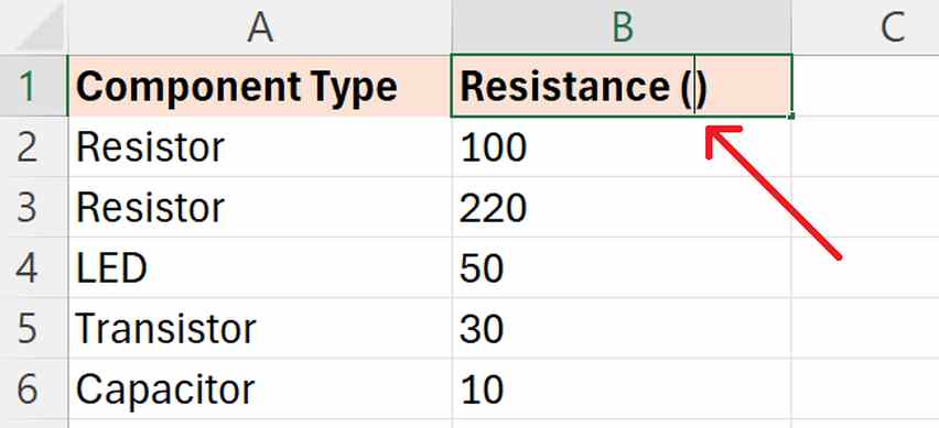
1. Navigate to the Cell Where You Want to Add the Symbol

Click on the specific cell where you wish to add a symbol. In our example, we will click on the cell with the header “Resistance ( )” and position the cursor precisely in the middle of the parentheses. 

This will prepare us to insert the ohm symbol, indicating that the data below are measured in ohms.

2. Access the Symbol Menu

Go to the ‘Insert’ tab on the Excel menu bar and select the ‘Symbol’ option from the ‘Symbols’ group. This opens the Symbol dialog box where we can choose various characters. 

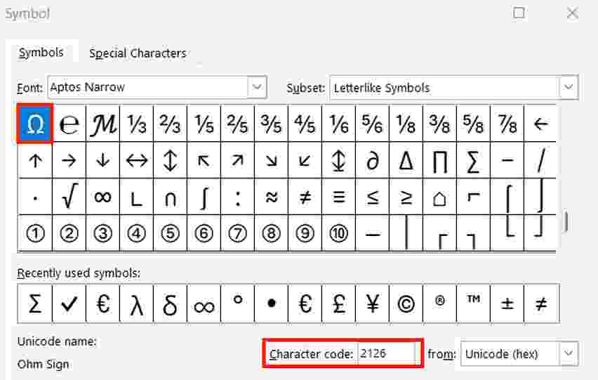
3. Find and Select the Ohm Symbol

In the Symbol dialog box, enter “2126” in the ‘Character code’ box to quickly locate the ohm symbol (Ω). Select it by clicking on it. 

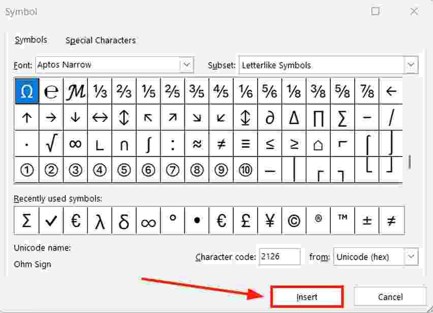
4. Insert the Ohm Symbol into the Cell

Click the ‘Insert’ button in the Symbol dialog box to place the ohm symbol into the selected cell. 

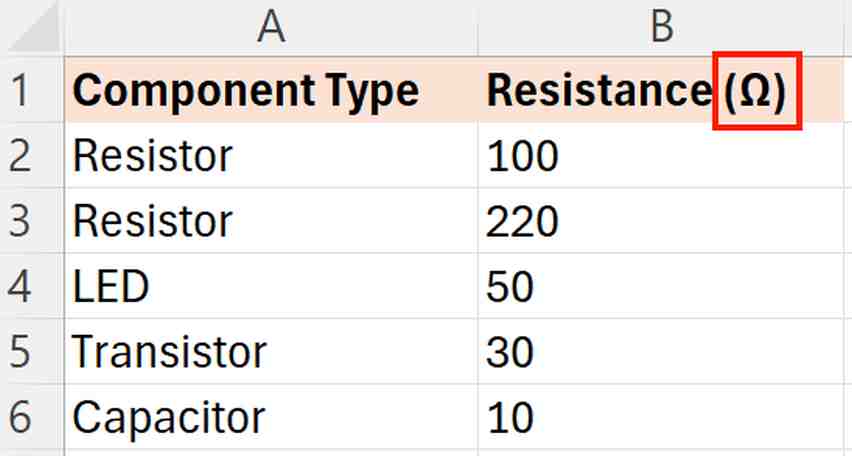
We will now see that our header changes from “Resistance ( )” to “Resistance (Ω)”, accurately representing the measurement unit for resistance.

We hope that you now have a better understanding of making an ohm symbol in Excel. If you enjoyed this article, you might also like our articles on how to insert a sigma symbol in Excel and how to add an approximate symbol in Excel.