Free Payback Period Calculator for Excel (Easiest Way in 2025)
In this article, we will show you how to create a payback period calculator in Excel. Simply follow the process below.
Free Payback Calculator for Excel
Get a copy of our free payback calculator for Excel by downloading it here.
How to Create a Payback Calculator in Excel
Follow the steps below to create a payback calculator in Excel.
1. Set up the Spreadsheet with Necessary Input Fields
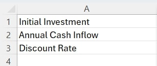
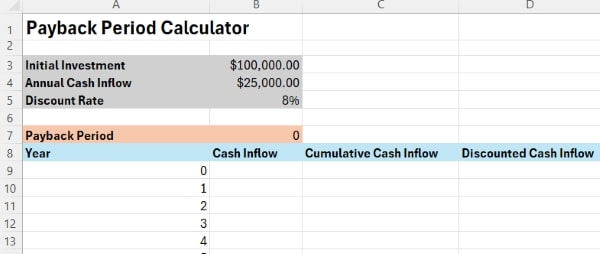
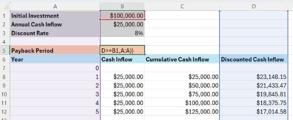
Create a new Excel spreadsheet. In cells A1 to A3, list out the key inputs needed to calculate the payback period: Initial Investment, Annual Cash Inflow, and Discount Rate.
2. Enter the Sample Data
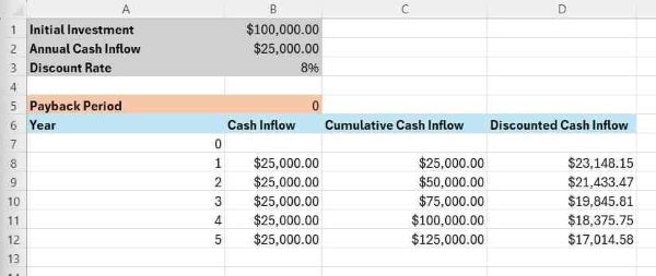
In cell B1, enter $100,000 for the Initial Investment. In B2, enter $25,000 for the Annual Cash Inflow. In B3, enter 8% for the Discount Rate.

3. Set up the Calculation Table
Starting in cell A7, create a table with columns for Year, Cash Inflow, Cumulative Cash Inflow, and Discounted Cash Inflow. In column A, have the year numbers increment down the rows, starting at 0.
4. Calculate the Annual Cash Inflow
In cell B8, enter the formula =$B$2 to reference the Annual Cash Inflow input.
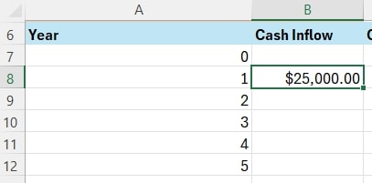
Drag this formula down to the remaining cells in the Cash Inflow column.
5. Calculate the Cumulative Cash Inflow
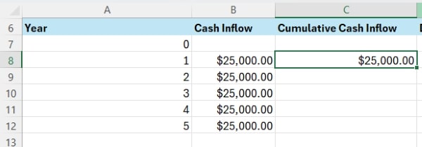
In cell C8, enter the formula =C7+B8 to add the current year’s cash inflow (B8) to the previous year’s cumulative cash inflow (C7). Drag this formula down to the remaining cells in the Cumulative Cash Inflow column.
6. Implement Discounting
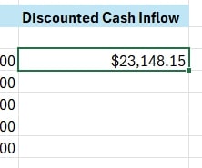
In cell D8, enter the formula =B8/(1+$B$3)^A8 to calculate the Discounted Cash Inflow. This divides the annual Cash Inflow (B8) by (1+discount rate)^year, where the discount rate is referenced from cell B3 and the year number is in column A.
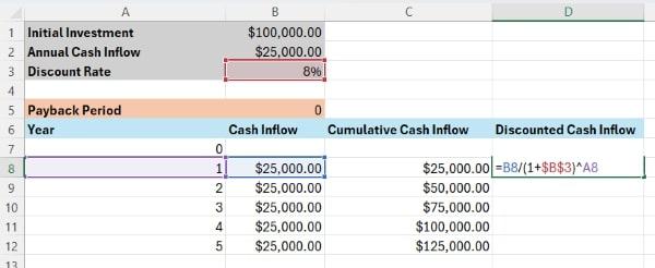
Drag this formula down to the remaining cells in the Discounted Cash Inflow column.
7. Determine the Payback Period
In cell B5, enter the formula =MIN(IF(D:D>=B1,A:A)) to find the first year where the Cumulative Cash Inflow (column D) exceeds the Initial Investment (cell B1). This is the payback period. Use conditional formatting to highlight the cell in column D where this occurs.
8. Make the Calculator Dynamic
Test the calculator by changing the input values in cells B1, B2, and B3. The calculation table and payback period should automatically update. Consider adding data validation to the input cells (e.g., to ensure the Initial Investment and Annual Cash Inflow are positive numbers and the Discount Rate is a percentage).

9. Format and Label
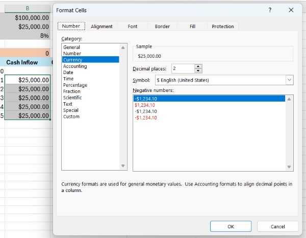
Apply appropriate formatting to the spreadsheet. For example, use currency formatting ($) for monetary values in columns B, C, D, and E. Add borders around the input cells and calculation table. Label cell B5 as “Payback Period”. Adjust column widths and font sizes to make the calculator fit nicely on the screen.
We hope that you now have a better understanding of how to set up a payback period calculator in Excel.
If you enjoyed this article, you might also like our article on how to set up a depreciation calculator in Excel and our article on how to reference a sheet name in Excel.

