Filter Unique Values in Excel (Easiest Way in 2025)
In this article, you will learn how to filter unique values in Excel from your data.
Filter Unique Values in Excel Using the Remove Duplicates Feature
Follow the steps below to filter unique values in Excel and ensure accurate data set without duplication.
1. Select the Entire Data Range Including Headers You Would Like to Filter
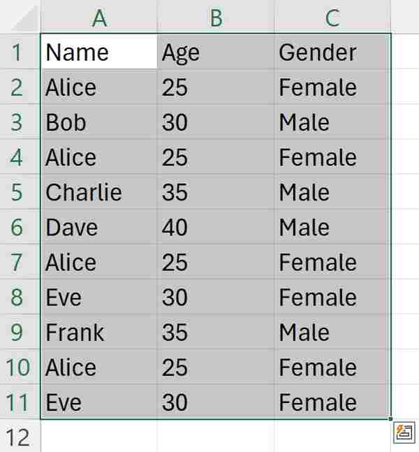
For example, click and drag your mouse to select the entire dataset, including the column headers (A1:C11). This step ensures that all the data within the specified range will be included when we filter for unique values.
2. Navigate to the “Data” Tab on the Excel Ribbon
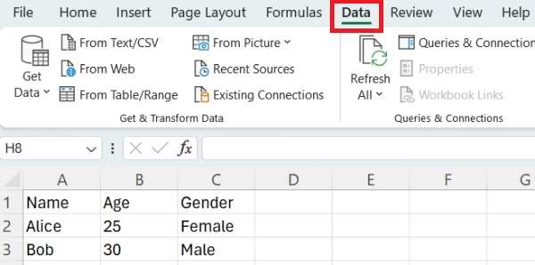
At the top of the Excel window, you’ll see a series of tabs. Click on the “Data” tab. This tab contains tools and commands related to data management and analysis.
3. Click on the “Remove Duplicates” Button in the Data Tab
In the “Data” tab, look for the “Data Tools” group. Within this group, you’ll find the “Remove Duplicates” button. Click on this button to open the “Remove Duplicates” dialog box.

4. Confirm the Columns to Filter for Unique Values
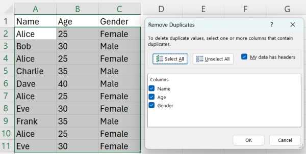
In the “Remove Duplicates” dialog box, Excel will automatically select all columns in your data range (Name, Age, Gender). These are the columns Excel will use to identify and remove duplicate rows.
5. Click “OK” to Apply the Filter for Unique Values
After confirming that the correct columns are selected, click the “OK” button in the “Remove Duplicates” dialog box.
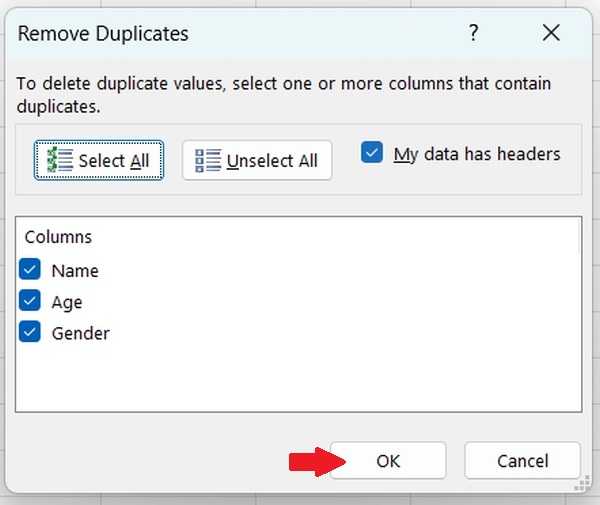
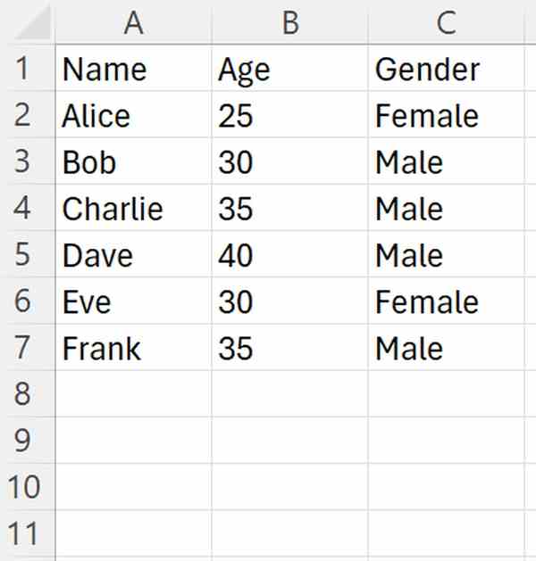
Excel will now apply the filter and remove any duplicate rows based on the entire row’s data.
Filter Unique Values in Excel Using Unique Function
To filter unique values in your Excel, you can use the Unique function. Here’s how to do it:
1. Choose a Cell to Display Unique Values
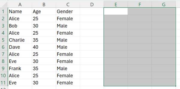
Identify the specific cell within your Excel worksheet where you want the unique values to be displayed after filtering (E1:G11). This cell acts as the destination for the results of the UNIQUE function. You can click directly into the cell to select it.
2. Initiate the Formula with “=” Sign
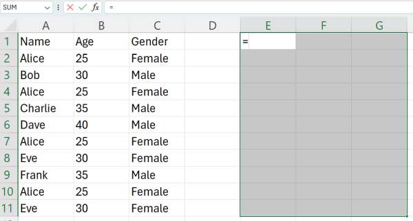
In the selected cell, start creating a formula by typing the equal sign “=” on your keyboard. This signals to Excel that you’re about to enter a formula or function into the cell. You’ll need this step to prepare for using the UNIQUE function.
3. Start Using the UNIQUE Function
Continue building your formula by typing “UNIQUE(” immediately after the equal sign. This indicates that you want to use the UNIQUE function in Excel. The UNIQUE function will help you extract only the distinct values from your dataset, filtering out any duplicates.
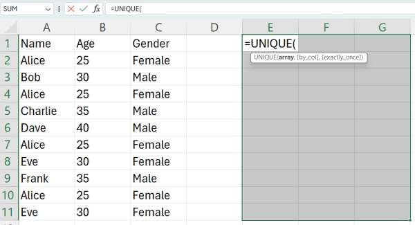
4. Specify Data Range for Extraction
Select the range of data from which you want to extract the unique values. This could be a single column or a larger range containing multiple columns (A1:C11). Click and drag to highlight the desired data range within your Excel worksheet.
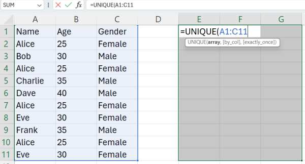
5. Close Function and Confirm Selection
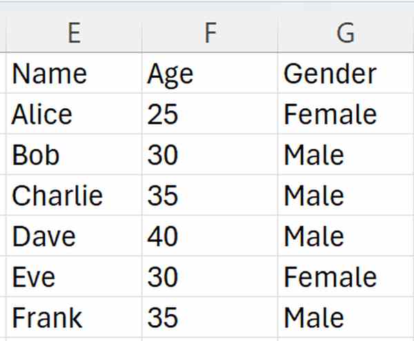
Complete the UNIQUE function by closing the parenthesis “)” and then press Enter on your keyboard. This action applies the function to the selected data range and displays the unique values in the cell you initially selected.
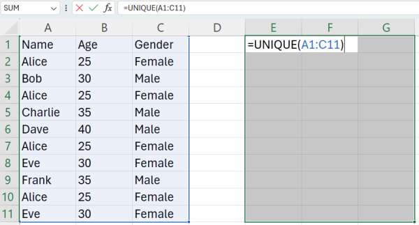
Your Excel worksheet will now show only the distinct values from your dataset.
We hope that you now know how to filter unique values in Excel. If you enjoyed this article, you might also like our article on how to count filtered rows in Excel or our article on how to filter a list in Excel.

