How to Filter Multiple Columns in Excel (Easiest Way in 2024)

In this article, you will learn how to filter multiple columns in Excel in order to organize and analyze data more effectively. Simply follow the steps below.

Filter Multiple Columns in Excel

Follow the process below to filter by multiple columns in Excel.

1. Select the Entire Dataset

Begin by selecting the entire dataset. Click on any cell within your data, then pressCtrl+A on your keyboard. This shortcut should select everything in your spreadsheet, all the rows and columns. 

If Ctrl+A doesn’t highlight everything, manually select the data by clicking and dragging from the top-left corner to the bottom-right corner, or by selecting entire columns using Ctrl+Spacebar.

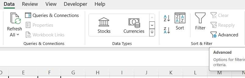
2. Go to the “Data” Tab

Look at the top of Excel. You’ll see different tabs. Click on the one that says “Data.” This is where you’ll find all sorts of things you can do with your data, including filtering.

3. Click on the “Filter” Button

In the “Data” tab, you’ll find a group called “Sort & Filter.” Inside that group, there’s a button that looks like a funnel. Click on that button. It’s called “Filter.” This will give you little arrows on top of your columns, which helps you filter your data.

4. Click on the Filter Arrow of the First Column You Want to Filter

Now, find the column you want to filter. At the top of that column, you’ll see a tiny arrow. Click on it. This opens up a menu where you can choose how to filter your data in that column.

5. Choose the Criteria You Want to Filter By

After clicking the arrow, you’ll see a menu with different options. You can choose specific things you want to see or hide in that column. It’s like telling Excel, “Show me only this stuff, please.”

6. Repeat Steps 4 and 5 for each Additional Column You Want to Filter

If you have more columns you want to filter, don’t worry. Just go to the next column you want to filter, click its arrow, and choose what you want to see or hide there. You can do this for as many columns as you need.

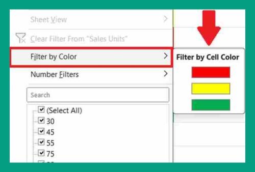
7. Clear Filters (Optional)

If you want to see all your data again without any filters, that’s easy. Just go back to the “Data” tab, find the “Sort & Filter” group, and click on “Clear.” This removes all the filters you’ve applied.

8. Close the Filter Menu (Optional)

Once you’ve finished filtering and you’re happy with what you see, you can close the filter menu. Just click on the arrow again, or click anywhere outside the menu.

9. Save your Changes

Last but not least, don’t forget to save your work. Click on the little floppy disk icon at the top, or go to “File” and then “Save.” This makes sure all your filtered data stays the way you want it.

Filter Multiple Columns in Excel Using Advanced Filter

Follow the steps below to filter multiple columns in Excel using the Advanced filter. 

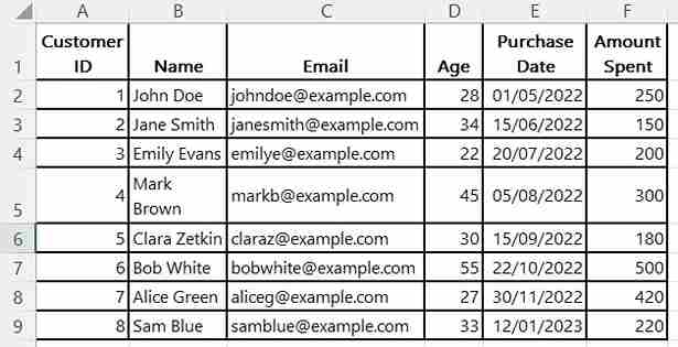
1. Organize Your Data in Columns with Clear Headers

Enter your data starting from cell A1 for headers: Customer ID, Name, Email, Age, Purchase Date, and Amount Spent. Fill the rows below with corresponding customer data starting from A2 to H8.

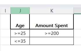
2. Create a Criteria Range for Filtering

Set up your criteria range starting at cell J1. In cells J1 and K1, enter the headers ‘Age’ and ‘Amount Spent’, respectively. Below these headers, input the filtering conditions:

In cells J2 and J3, type “>=25” and “<=35” to filter ages between 25 and 35.

In cell K2, type “>=200” to target customers who spent at least $200.

This configuration allows you to filter for customers within a specific age range and spending threshold.

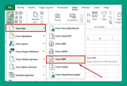
3. Access the Advanced Filter Dialog Box from the Data Tab

Click any cell within your data set (e.g., A2). Navigate to the ‘Data’ tab on the ribbon and select ‘Advanced’ in the ‘Sort & Filter’ group to open the Advanced Filter dialog box.

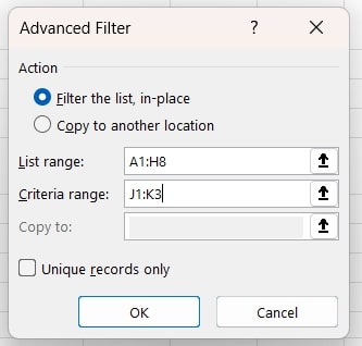
4. Configure List and Criteria Ranges in the Advanced Filter

In the Advanced Filter dialog box, choose ‘Filter the list, in-place’ or ‘Copy to another location’. For the ‘List range’, select A1:H8 which covers your entire data set. For the ‘Criteria range’, select J1:K3 which includes the headers and their conditions.

5. Apply the Filter to Display Matching Data Rows

After setting your list and criteria ranges, click ‘OK’. If you are filtering in place, your original data view will update to show only those rows meeting your criteria.

We hope that you now have a better understanding of how to filter multiple columns in Excel. If you enjoyed this article, you might also like our article on how to filter in Excel based on a list and our article on how to filter horizontally in Excel.